Thursday, November 29, 2012
OGPSS - The ARPA-E 2012 Awards
The Department of Energy has just announced the projects that have been selected for funding in the next round of the ARPA-E program. (This is the Advanced Research Projects Agency-Energy, first funded in 2009, to, inter alia, "focus on creative “out-of-the-box” transformational energy research that industry by itself cannot or will not support due to its high risk but where success would provide dramatic benefits for the nation".) There are some 66 projects on the list, which is broken down into eleven different focus areas. These are the technologies that the ARPA-E program is betting some $130 million on, as sources of future energy supply or savings. It is worth taking a quick glance through the topics to see what is considered important and likely of success.
The two largest areas of funding are Advanced Fuels and Grid Modernization, both of which get around $24 million or 18% of the pie. This is split among 13 fuel projects, and 9 grid-related projects. With the growing supply of natural gas that is coming from the developing shale gas reserves in the country, it is perhaps no surprise to see that methane conversion to liquid fuel captures the largest part of the fuel funding this year, being the theme of nine of the awards.
The largest of the fuel awards goes to Allylix a company that specializes in terpenes, and who is tasked with turning these into a viable aviation fuel. Specific genes needed for terpene production are extracted from a biosource, and then optimized for use in a yeast host. The optimization is an engineered change that can increase product yield several hundred fold (according to their website). From that point there is a fermentation process, and then a recovery and purification of the liquid fuel, which is stated to be already commercially viable.
There is only one algae award this year, to Cornell for $910 k, and they will look at using light fibers in a small reactor as a means of improving economics. After having looked into this process I am prone to disagree that smaller is better (if you are going to generate hundreds of thousands of barrels a day you need large systems, and anything on a smaller scale is hardly worthwhile). Further there are issues with engineered light paths, but they will no doubt find those out as they carry on with their work.
The “different” program in this effort is for $1.8 million which is being given to Plant Sensory Systems to develop a high-output, low-input beet plant for sugar production.
There are just two awards for Advanced Vehicles, one to Electron Energy Corp to produce better permanent magnets that don’t rely on rare-earths, and one to United Technologies to improve efficiency by using laser deposition of alternate layers of copper and insulation in a new electric motor design. This will also reduce rare-earth dependence. They roughly split $5.6 million.
The $5.3 million for improving building efficiency goes to California, and is split with two awards to Lawrence Berkeley and one to Stanford. Each has a project on using coatings to alter the thermal transfer to the buildings and cars, while Lawrence Berkeley also gets almost $2 million for modeling studies of building heat losses.
The $10 million for carbon capture is split four ways, with two awards (to Arizona State and Dioxide Materials) for electrochemical systems that will generate new fuels from the carbon dioxide output of power plants, while the University of Massachusetts at Lowell is developing (for $3 million) a catalyst that will also combine sunlight, CO2 and water into a fuel precursor.
The fourth award is to the University of Pittsburg (at $2.4 million) for a way to thicken liquid CO2 either as a way of improving EOR, or as a substitute for water in hydrofracking. I can’t quite see the advantage of a thicker fluid for use in EOR, since the hope, surely, is to have a very low viscocity fluid that can more easily penetrate into the formation and mix with the oil, but the application in fracking is intriguing.
The emphasis with the investments in Grid Modernization (the co-largest topic) is on improving switchgear (five awards). In addition there are two awards for modeling, one on improved instrumentation and one to Grid Logic ($3.8 million) for developing a new super-conducting wire for power transmission.
There are two awards, both for $2 million, in the “Other” category. One is to MIT for a water purification system, wile the other is to Harvard. This latter is for a “self-repairing” coating that can be applied to water and oil pipes to reduce friction and thus lower pumping costs. The old fall-back on this was Teflon, which could be very effective, but any particulate matter in the fluid will erode this over time, so the “self-healing” aspect could be worthwhile, since it might allow a much thinner liner.
The $18.76 million for Renewable Energy projects is distributed to wind, sun and water energies, with two projects in waves where Brown University will be building a new underwater wing to capture flowing water energy, and Sea Engineering, who will be developing a better buoy for acquiring data for tidal energy potential assessment. Wind is down to a two projects, one, which seems a bit regressive, is to GE who will develop fabric blades for wind turbines for $3.7 million. A similar amount is going to Georgia Tech to develop a vertical axis turbine. The remaining six projects deal with solar power of which the most interesting, perhaps, is that at Cal Tech which is going to look into splitting light into its different color bands (think prism) before using them to improve device efficiency. We have seen that converting white light electronically to the narrow optimal color band can have dramatic effects on improving algae growth rates, for example, but it requires a bit more refinement to achieve the narrow division than, I suspect, will be possible optically.
The section that will invest $12 million in Stationary Energy Storage is funding 8 projects looking at different battery technologies. The largest investment ($4 million) is going to Alveo Energy, which has an intriguing entry in Find the Company. It was apparently only founded this year. The technology that it is chasing involves using Prussian Blue dye as the active ingredient in the battery.
The other “out of the ordinary” award is to Tai Yang which is affiliated with Florida State University. Superconductivity Center. The $2.15 million award is to develop a method for storing energy in a high-power superconducting cable.
Pratt and Whitney get two of the three Stationary Generation awards, the first for $650k is to develop a continuous detonation gas turbine, while the second, for $600 k is for work on an ultra-high temperature gas turbine. The University of North Dakota gets the third award to look at developing air cooling for power plants.
The $9.5 million for Thermal Energy Storage is split five ways, with three awards for the development of power from the waste heat in existing systems, one to the NREL for a solar thermal electric generator, and one to Georgia Tech for a solar fuels reactor using liquid metals.
When it comes to finding answers to Transportation Energy Storage the Agency is committing $15.3 million to seven projects. Six of these deal with battery development. (A123 Systems who previously received a $249 million federal grant to develop electric car batteries recently went bankrupt.) Two of the awards, to Georgia Tech and to UC Santa Barbara will seek to combine super-capacitor design with battery capabilities, while the Palo Alto Research Center will use a printing process to construct batteries.
Ceramatec is being funded, at $2.1 million, to develop a solid-state fuel cell using low-cost materials.
There is a clear change in emphasis from earlier years reflecting, no doubt, the results from ongoing research, as well as the obvious change that the current natural gas availability is allowing in developing technical advances for the future. It should, however, be born in mind that while some of these will likely prove to be quite successful, it will still take perhaps a decade before any of them can be anticipated to have any significant impact on the market.
Read more!
Sunday, November 25, 2012
Waterjetting 3d - High-pressure pump flow and pressure
When I first began experimenting with a waterjet system back in 1965 I used a pump that could barely produce 10,000 psi. This limited the range of materials that we could cut (this was before the days when abrasive particles were added to the jet stream) and so it was with some anticipation that we received a new pump, after my move to Missouri in 1968. The new, 60-hp pump came with a high-pressure end that delivered 3.3 gpm at 30,000 psi. which meant that a 0.027 inch diameter orifice in the nozzle was needed to achieve full operating pressure.
However I could also obtain (and this is now a feature of a number of pumps from different suppliers) a second high-pressure end for the pump. By unbolting the first, and attaching the second, I could alter the plunger and cylinder diameters so that, for the same drive and motor rpm, the pump would now deliver some 10 gpm at a flow rate of 10 gpm. This flow, at the lower pressure, could be used to feed four nozzles, each with a 0.029 inch diameter.
 Figure 1. Delivery options from the same drive train with two different high-pressure ends.
The pressure range that this provided covers much of the range that was then available for high-pressure pumping units using the conventional multi-piston connection through a crankshaft to a single drive motor. Above that pressure it was necessary to use an intensifier system, which I will cover in later posts.
However there were a couple of snags in using this system to explore the cutting capabilities of waterjet streams in a variety of targets. The first of these was when the larger flow system was attached to the unit. In order to compare “apples with apples” at different pressures some of the tests were carried out with the same nozzle orifice. But the pump drive motor was a fixed speed unit which produced the same 10 gpm volume flow out of the delivery manifold regardless of delivery pressure (within the design limits). Because the single small nozzle would only handle a quarter of this flow, at that pressure (see table from Waterjetting 1c) the rest of the water leaving the manifold needed an alternate path.
Figure 1. Delivery options from the same drive train with two different high-pressure ends.
The pressure range that this provided covers much of the range that was then available for high-pressure pumping units using the conventional multi-piston connection through a crankshaft to a single drive motor. Above that pressure it was necessary to use an intensifier system, which I will cover in later posts.
However there were a couple of snags in using this system to explore the cutting capabilities of waterjet streams in a variety of targets. The first of these was when the larger flow system was attached to the unit. In order to compare “apples with apples” at different pressures some of the tests were carried out with the same nozzle orifice. But the pump drive motor was a fixed speed unit which produced the same 10 gpm volume flow out of the delivery manifold regardless of delivery pressure (within the design limits). Because the single small nozzle would only handle a quarter of this flow, at that pressure (see table from Waterjetting 1c) the rest of the water leaving the manifold needed an alternate path.
 Figure 2. Positive displacement pump with a bypass circuit.
This was provided through a bypass circuit (Figure 2) so that, as the water left the high-pressure manifold it passed through a “T” connection, with the perpendicular channel to the main flow carrying the water back to the original water tank. A flow control valve on this secondary circuit would control the orifice size the water had to pass through to get back to the water tank, thereby adjusting the flow down the main line to the nozzle, and concurrently controlling the pressure at which the water was driven.
Thus, when a small nozzle was attached to the cutting lance most of the flow would pass through the bypass channel. While this “works” when the pump is being used as a research tool, it is a very inefficient way of operating the pump. Bear in mind that the pump is being run at full pressure and flow delivery, but only 25% of the flow is being sent to the cutting system. This means that you are wasting 75% of the power of the system. There are a couple of other disadvantages that I will discuss later in more detail, but the first is that the passage through the valve will heat the water a little. Keep recirculating the water over time and the overall temperature will rise to levels that can be of concern (it melted a couple of fittings on one occasion). The other is that if you are using a chemical treatment in the water then the recirculation can quite rapidly affect the results, usually negatively.
It would be better if the power of the pump were fully used in delivering the water flow rate required for the cutting conditions under which the pump was being used. With a fixed size of pistons and cylinders this can be achieved, to an extent, by changing the rotation speed of the drive shaft. This can, in turn, be controlled through use of a suitable gearbox between the drive motor and the main shaft of the pump. As the speed of the motor increases, so the flow rate also rises. For a fixed nozzle size this means that the pressure will also rise. And the circuit must therefore contain a safety valve (or two) that will open at a designated pressure to stop the forces on the pump components from rising too high.
Figure 2. Positive displacement pump with a bypass circuit.
This was provided through a bypass circuit (Figure 2) so that, as the water left the high-pressure manifold it passed through a “T” connection, with the perpendicular channel to the main flow carrying the water back to the original water tank. A flow control valve on this secondary circuit would control the orifice size the water had to pass through to get back to the water tank, thereby adjusting the flow down the main line to the nozzle, and concurrently controlling the pressure at which the water was driven.
Thus, when a small nozzle was attached to the cutting lance most of the flow would pass through the bypass channel. While this “works” when the pump is being used as a research tool, it is a very inefficient way of operating the pump. Bear in mind that the pump is being run at full pressure and flow delivery, but only 25% of the flow is being sent to the cutting system. This means that you are wasting 75% of the power of the system. There are a couple of other disadvantages that I will discuss later in more detail, but the first is that the passage through the valve will heat the water a little. Keep recirculating the water over time and the overall temperature will rise to levels that can be of concern (it melted a couple of fittings on one occasion). The other is that if you are using a chemical treatment in the water then the recirculation can quite rapidly affect the results, usually negatively.
It would be better if the power of the pump were fully used in delivering the water flow rate required for the cutting conditions under which the pump was being used. With a fixed size of pistons and cylinders this can be achieved, to an extent, by changing the rotation speed of the drive shaft. This can, in turn, be controlled through use of a suitable gearbox between the drive motor and the main shaft of the pump. As the speed of the motor increases, so the flow rate also rises. For a fixed nozzle size this means that the pressure will also rise. And the circuit must therefore contain a safety valve (or two) that will open at a designated pressure to stop the forces on the pump components from rising too high.
 Figure 3. Output flows from a triplex (3-piston) pump in gpm, for varying piston size and pump rotation speed. Note that the maximum operating pressure declines as flow increases, to maintain a safe operating force on the crankshaft.
The most efficient way of removing different target materials varies with the nature of that material. But it should not be a surprise that neither a flow rate of 10 gpm at 10,000 psi, nor a flow rate of 3.3 gpm at 30,000 psi gave the most efficient cutting for most of the rock that we cut in those early experiments.
To illustrate this with a simple example: consider the case where the pump was used configured to produce 3.3 gpm at pressures up to 30,000 psi. At a nozzle diameter of 0.025 inches the pump registered a pressure of 30,000 psi for full flow through the nozzle. At a nozzle diameter of 0.03 inches the pump registered a pressure of 20,000 psi at full flow, and at a nozzle diameter of 0.04 inches the pressure of the pump was 8,000 psi. (The numbers don’t quite match the table because of water compression above 15,000 psi). Each of these jets was then used to cut a slot across a block of rock, cutting at the same traverse speed (the relative speed of the nozzle over the surface), and at the same distance between the nozzle and the rock. The depth of the cut was then averaged over the cut length.
Figure 3. Output flows from a triplex (3-piston) pump in gpm, for varying piston size and pump rotation speed. Note that the maximum operating pressure declines as flow increases, to maintain a safe operating force on the crankshaft.
The most efficient way of removing different target materials varies with the nature of that material. But it should not be a surprise that neither a flow rate of 10 gpm at 10,000 psi, nor a flow rate of 3.3 gpm at 30,000 psi gave the most efficient cutting for most of the rock that we cut in those early experiments.
To illustrate this with a simple example: consider the case where the pump was used configured to produce 3.3 gpm at pressures up to 30,000 psi. At a nozzle diameter of 0.025 inches the pump registered a pressure of 30,000 psi for full flow through the nozzle. At a nozzle diameter of 0.03 inches the pump registered a pressure of 20,000 psi at full flow, and at a nozzle diameter of 0.04 inches the pressure of the pump was 8,000 psi. (The numbers don’t quite match the table because of water compression above 15,000 psi). Each of these jets was then used to cut a slot across a block of rock, cutting at the same traverse speed (the relative speed of the nozzle over the surface), and at the same distance between the nozzle and the rock. The depth of the cut was then averaged over the cut length.
 Figure 4. Depth of cut into sandstone, as a function of nozzle diameter and jet pressure.
If the success of the jet cut is measured by the depth of the cut achieved, then the plot shows that the optimal cutting condition would likely be achieved with a nozzle diameter of around 0.032 inches, with a jet pressure of around 15,000 psi.
This cut is not made at the highest jet pressure achievable, nor is it at the largest diameter of the flow tested. Rather it is at some point in between, and it is this understanding, and the ability to manipulate the pressures and flow rates of the waterjets produced from the pump that makes it more practical to optimize pump performance through the proper selection of gearing, than it was when I got that early pump.
This does not hold true just for using a plain waterjet to cut into rock, but it has ramifications in other ways of using both plain and abrasive-laden waterjets, and so we will return to the topic as this series continues.
Figure 4. Depth of cut into sandstone, as a function of nozzle diameter and jet pressure.
If the success of the jet cut is measured by the depth of the cut achieved, then the plot shows that the optimal cutting condition would likely be achieved with a nozzle diameter of around 0.032 inches, with a jet pressure of around 15,000 psi.
This cut is not made at the highest jet pressure achievable, nor is it at the largest diameter of the flow tested. Rather it is at some point in between, and it is this understanding, and the ability to manipulate the pressures and flow rates of the waterjets produced from the pump that makes it more practical to optimize pump performance through the proper selection of gearing, than it was when I got that early pump.
This does not hold true just for using a plain waterjet to cut into rock, but it has ramifications in other ways of using both plain and abrasive-laden waterjets, and so we will return to the topic as this series continues.


Read more!
Sunday, November 18, 2012
Waterjettting 3c - Pressure Washers
It is sometimes easy, in these days when one can go down to the local hardware store and buy a Pressure Washer that will deliver flow rates of a few gallons a minute (gpm) at pressures up to 5,000 psi, to forget how recently that change came about.
One learns early in the day that the largest volume market for pressurized water systems lies in their use as a domestic/commercial cleaning tool. But even that development has happened within my professional lifetime. It is true that one can go back to the mid-1920’s and find pictures of pressure washers being used for cleaning cars, and not only did Glark Gable pressure-paint his fences, but I have seen an old film of him pressure washing his house in the 1930’s.
 Figure 1. Pressure washing a car in 1928 (courtesy FMC and Industrial Cleaning Technology by Harrington).
Yet it was not a common tool. The first automated car wash dates from 1947, while the average unit today will service around 71,000 cars a year, and there are about 22,000 units in the country.
When I first went to the Liquid Waste Haulers show in Nashville (now the Pumper and Cleaner Environmental Expo International) the dominant method for cleaning sewer lines was with a spinning chain or serrated saw blade of the Roto-Rooter type. Over the past two decades this has been supplanted by the growth of an increasing number of pressurized washer systems, than can be sent down domestic and commercial sewer lines to clean out blockages and restore flow. As in a number of other applications the pressure of the jet system can be adjusted so that the water can cut through the obstruction, without doing damage to the enclosing pipe. The technology has even acquired its own term, that of Moleing a line. And, for those interested there are a variety of videos that can now be viewed on Youtube showing some of the techniques. (see for example this video). Unfortunately just because a tool is widely available, and simple to assemble, does not mean that it is immediately obvious how best to use it, nor that it is safe to do so, and I will comment on some sensible precautions to take, when I deal with the use of cleaning systems later in this series.
For now, however, I would like to just discuss the use of pressure washers from the aspect that they are the lower end of the range in which the pressure of the water is artificially raised to some level in order to do constructive work. At this level of pressure it is quite common to hook the base pump up to the water system at the house or plant. Flow rates are relatively low, and can be met from a tap. The pressure of the water in the line is enough to keep water flowing, without problems, into the low-pressure side of the pump, although this can be a problem at higher pressures and flows, as will be discussed in the article on the use of 10,000 psi systems.
The typical pressure washer that is used for domestic cleaning will operate at flow rates of around 2-5 gpm and at pressures up to 5,000 psi. Below 2,000 psi the units are often driven by electric motors, while above that the pumps are driven by small gasoline engines. In both cases the engine will normally rotate at a constant speed. With the typical unit having three pistons, the pump will deliver a relatively constant volume of water into the delivery hose.
There are two ways of controlling the pressure that the pump produces. Because the flow into the high-pressure size of the pump is constant, the pressure is generally controlled by the size of the orifice through which the water must then flow. These nozzle sizes are typically set by the manufacturer, with the customer buying a suite of nozzles that are designed to produce jets of different shape, and occasionally pressure.
An alternative way of controlling pressure is to add a small by-pass circuit to the delivery hose, so that, by opening and closing a valve in that line, the amount of water that flows to the delivery nozzle will be controlled, and with that flow so also will the delivery pressure.
Because the three pistons that typically drive water from the low-pressure side of the pump to the high pressure side are attached at 120 degree increments around the crankshaft, and because the pistons must each compress the water at the beginning of the stroke, and bring it up to delivery pressure before the valve opens, there is a little fluctuation in the pressure that is delivered by the pump.
In a later article I will write about some of the advantages of having a pulsating waterjet delivery system (as well as some of the disadvantages if you do it wrong – I seem to remember a piston being driven through the end of a pump cylinder in less than five-minutes of operation in one of the early trials of one such system). In some applications that pulsation can be an advantage, particularly in cleaning, but in others it can reduce the quality of the final product. With less expensive systems however it is normally not possible to eradicate this pulsation.
The Cleaning Equipment Manufacturer’s Association (CEMA – now the Cleaning Equipment Trade Association funded the Underwriters Laboratory to write a standard for the industry (UL 1776) almost 20-years ago. That standard is now being re-written to conform to international standards that are being developed for this industry. There are also standards for the quality of surfaces after they have been cleaned, but these largely deal with cleaning operations at higher pressures, and so will form a topic for future posts, when discussing cleaning at pressures above 10,000 psi.
Sadly although pressure washers are now found almost everywhere, very few folk fully understand enough about how a waterjet works to make their use most effective. Because most operators use a fan jet to cover the surfaces that they are cleaning, the pressure loss moving away from the nozzle can be very rapid. A simple test I run with most of my student classes is to have them direct the jet at a piece of mildewed concrete. Despite the fact that I have shown them, in class, that a typical cleaning nozzle produces a jet that is only effective for about four inches, most students start by holding the nozzle about a foot from the surface. All it is doing is getting the surface wet, and promising a slow, ineffective cleaning operation.
No matter how efficient the pump, if the water is not delivered effectively through the delivery system and nozzle, then the investment is not being properly utilized. It is a topic I will return to on more than one occasion.
Figure 1. Pressure washing a car in 1928 (courtesy FMC and Industrial Cleaning Technology by Harrington).
Yet it was not a common tool. The first automated car wash dates from 1947, while the average unit today will service around 71,000 cars a year, and there are about 22,000 units in the country.
When I first went to the Liquid Waste Haulers show in Nashville (now the Pumper and Cleaner Environmental Expo International) the dominant method for cleaning sewer lines was with a spinning chain or serrated saw blade of the Roto-Rooter type. Over the past two decades this has been supplanted by the growth of an increasing number of pressurized washer systems, than can be sent down domestic and commercial sewer lines to clean out blockages and restore flow. As in a number of other applications the pressure of the jet system can be adjusted so that the water can cut through the obstruction, without doing damage to the enclosing pipe. The technology has even acquired its own term, that of Moleing a line. And, for those interested there are a variety of videos that can now be viewed on Youtube showing some of the techniques. (see for example this video). Unfortunately just because a tool is widely available, and simple to assemble, does not mean that it is immediately obvious how best to use it, nor that it is safe to do so, and I will comment on some sensible precautions to take, when I deal with the use of cleaning systems later in this series.
For now, however, I would like to just discuss the use of pressure washers from the aspect that they are the lower end of the range in which the pressure of the water is artificially raised to some level in order to do constructive work. At this level of pressure it is quite common to hook the base pump up to the water system at the house or plant. Flow rates are relatively low, and can be met from a tap. The pressure of the water in the line is enough to keep water flowing, without problems, into the low-pressure side of the pump, although this can be a problem at higher pressures and flows, as will be discussed in the article on the use of 10,000 psi systems.
The typical pressure washer that is used for domestic cleaning will operate at flow rates of around 2-5 gpm and at pressures up to 5,000 psi. Below 2,000 psi the units are often driven by electric motors, while above that the pumps are driven by small gasoline engines. In both cases the engine will normally rotate at a constant speed. With the typical unit having three pistons, the pump will deliver a relatively constant volume of water into the delivery hose.
There are two ways of controlling the pressure that the pump produces. Because the flow into the high-pressure size of the pump is constant, the pressure is generally controlled by the size of the orifice through which the water must then flow. These nozzle sizes are typically set by the manufacturer, with the customer buying a suite of nozzles that are designed to produce jets of different shape, and occasionally pressure.
An alternative way of controlling pressure is to add a small by-pass circuit to the delivery hose, so that, by opening and closing a valve in that line, the amount of water that flows to the delivery nozzle will be controlled, and with that flow so also will the delivery pressure.
Because the three pistons that typically drive water from the low-pressure side of the pump to the high pressure side are attached at 120 degree increments around the crankshaft, and because the pistons must each compress the water at the beginning of the stroke, and bring it up to delivery pressure before the valve opens, there is a little fluctuation in the pressure that is delivered by the pump.
In a later article I will write about some of the advantages of having a pulsating waterjet delivery system (as well as some of the disadvantages if you do it wrong – I seem to remember a piston being driven through the end of a pump cylinder in less than five-minutes of operation in one of the early trials of one such system). In some applications that pulsation can be an advantage, particularly in cleaning, but in others it can reduce the quality of the final product. With less expensive systems however it is normally not possible to eradicate this pulsation.
The Cleaning Equipment Manufacturer’s Association (CEMA – now the Cleaning Equipment Trade Association funded the Underwriters Laboratory to write a standard for the industry (UL 1776) almost 20-years ago. That standard is now being re-written to conform to international standards that are being developed for this industry. There are also standards for the quality of surfaces after they have been cleaned, but these largely deal with cleaning operations at higher pressures, and so will form a topic for future posts, when discussing cleaning at pressures above 10,000 psi.
Sadly although pressure washers are now found almost everywhere, very few folk fully understand enough about how a waterjet works to make their use most effective. Because most operators use a fan jet to cover the surfaces that they are cleaning, the pressure loss moving away from the nozzle can be very rapid. A simple test I run with most of my student classes is to have them direct the jet at a piece of mildewed concrete. Despite the fact that I have shown them, in class, that a typical cleaning nozzle produces a jet that is only effective for about four inches, most students start by holding the nozzle about a foot from the surface. All it is doing is getting the surface wet, and promising a slow, ineffective cleaning operation.
No matter how efficient the pump, if the water is not delivered effectively through the delivery system and nozzle, then the investment is not being properly utilized. It is a topic I will return to on more than one occasion.

Read more!
Thursday, November 15, 2012
OGPSS - Global oil demand and Iranian production
One of the headlines this week has come from the IEA Report that suggests that the United States will be the top global oil producer in five years. Yet back in DeSoto Parish in Louisiana where the Haynesville Shale discovery in 2008 started the bonanza, revenues are now falling and school board budgets are being tightened as the end of the glory days are now beginning to appear.
Just this week Aubrey McClendon has said that Chesapeake’s prospects for oil in Ohio, where Chesapeake had high hopes for the Utica Shale, are now dim. It is easy to look at one of the large maps that the Oil and Gas Journal include in their print editions, showing all the shale deposits in the United States, and to be carried away (as the IEA apparently are) with the vast acreage that is shaded on the map. Unfortunately, as we are seeing, reality tells another story. The size of the resources have been measured in the past, and with the best plays being given preference, the recognition of decline rates, and unprofitable wells have not yet been given the prominence in the popular press that they will ultimately draw.
 Figure 1. Shale Plays and Basins in the United States (Oil and Gas Journal)
It seems unrealistic to anticipate the levels of production that are now being projected for future North American production of oil. But, nevertheless, these do tend to crowd other stories on the subject out of the spotlight. And further, if the predictions for American production gains, even in the short term, turn out to be optimistic, then the impacts may be more exaggerated than is currently appreciated. Consider that OPEC now expect that North America will continue to provide the greatest y-o-y increase in supply over other nations, and there are, in fact, very few other nations that will be contributing that much more in the next year.
Figure 1. Shale Plays and Basins in the United States (Oil and Gas Journal)
It seems unrealistic to anticipate the levels of production that are now being projected for future North American production of oil. But, nevertheless, these do tend to crowd other stories on the subject out of the spotlight. And further, if the predictions for American production gains, even in the short term, turn out to be optimistic, then the impacts may be more exaggerated than is currently appreciated. Consider that OPEC now expect that North America will continue to provide the greatest y-o-y increase in supply over other nations, and there are, in fact, very few other nations that will be contributing that much more in the next year.
 Figure 2. Non-OPEC supply growth expressed as a year on year change. (OPEC November MOMR)
The MOMR notes that UK oil production has fallen below 1 mbd, for the first time since 1977, while Norway’s production has fallen to levels not seen since 1990. These numbers are part of an overall revision of non-OPEC production for 2013, which OPEC now sees as coming in, as follows.
Figure 2. Non-OPEC supply growth expressed as a year on year change. (OPEC November MOMR)
The MOMR notes that UK oil production has fallen below 1 mbd, for the first time since 1977, while Norway’s production has fallen to levels not seen since 1990. These numbers are part of an overall revision of non-OPEC production for 2013, which OPEC now sees as coming in, as follows.
 Figure 3. OPEC projections of non-OPEC production for 2013. (OPEC November MOMR)
In regard to OPEC production, the MOMR has, again, two tables for their production, with the first showing that based on secondary sources.
Figure 3. OPEC projections of non-OPEC production for 2013. (OPEC November MOMR)
In regard to OPEC production, the MOMR has, again, two tables for their production, with the first showing that based on secondary sources.
 Figure 4. OPEC production based on other sources ((OPEC November MOMR).
The tables show that Iranian oil production continues to decline, by around 47 kbd from September to October. Yet other sources are now reporting that both China and South Korea may have been helping Iran increase oil exports. As a result production may have increased 70 kbd, instead of declining, though the overall volume remains at around 2.7 mbd, of which exports rose from 1 mbd to 1.43 mbd.
When the “as reported directly” table is compared, Iran is shown to be still producing at around 3.7 mbd.
Figure 4. OPEC production based on other sources ((OPEC November MOMR).
The tables show that Iranian oil production continues to decline, by around 47 kbd from September to October. Yet other sources are now reporting that both China and South Korea may have been helping Iran increase oil exports. As a result production may have increased 70 kbd, instead of declining, though the overall volume remains at around 2.7 mbd, of which exports rose from 1 mbd to 1.43 mbd.
When the “as reported directly” table is compared, Iran is shown to be still producing at around 3.7 mbd.
 Figure 5. OPEC production based on direct communication with the producing country ((OPEC November MOMR).
Within Iran the government has partially reduced the subsidies that it was providing for gasoline, which initially reduced demand by about 50 tb/d, and flattening internal demand. But, as we enter the colder months OPEC is estimating that demand will again start to rise.
Concurrently Turkmenistan has stopped exporting natural gas to Iran. Normally Iran would increase imports, over the winter months to around 1 billion cu.ft/day (bcf/d), although this import is partly for geographic reasons, and Iran has, in the past, exported about 80% of the equivalent volume to Turkey. Iran has, apparently, suggested that Turkmenistan increase the delivery to 1.4 bcf/d, but since Turkmenistan can now get a good price for its gas from China, there is more of a debate this year over price, without agreement at the moment. Iran also swops around 35 mcf/d of natural gas with Armenia, in return for electric power.
As a way to try and work around the current sanctions, Iran has been changing to a scenario where it can move more of its oil using its own tankers. The country had been storing millions of barrels in part of this fleet, but that volume is being sold so that the vessels can, instead, haul oil. And there is the possibility that the insurance on these vessels has been “fiddled” to get around the burden imposed by sanctions.
Internally the sanctions are having considerable effect.
Figure 5. OPEC production based on direct communication with the producing country ((OPEC November MOMR).
Within Iran the government has partially reduced the subsidies that it was providing for gasoline, which initially reduced demand by about 50 tb/d, and flattening internal demand. But, as we enter the colder months OPEC is estimating that demand will again start to rise.
Concurrently Turkmenistan has stopped exporting natural gas to Iran. Normally Iran would increase imports, over the winter months to around 1 billion cu.ft/day (bcf/d), although this import is partly for geographic reasons, and Iran has, in the past, exported about 80% of the equivalent volume to Turkey. Iran has, apparently, suggested that Turkmenistan increase the delivery to 1.4 bcf/d, but since Turkmenistan can now get a good price for its gas from China, there is more of a debate this year over price, without agreement at the moment. Iran also swops around 35 mcf/d of natural gas with Armenia, in return for electric power.
As a way to try and work around the current sanctions, Iran has been changing to a scenario where it can move more of its oil using its own tankers. The country had been storing millions of barrels in part of this fleet, but that volume is being sold so that the vessels can, instead, haul oil. And there is the possibility that the insurance on these vessels has been “fiddled” to get around the burden imposed by sanctions.
Internally the sanctions are having considerable effect.


Although the government maintains that the official inflation rate is 25 percent, . . . with some analysts claiming that actual figures are double the government rate. In addition, unemployment has soared, with estimates stating that between 500,000 and 800,000 Iranians have lost their jobs. . . . . ."Business is drying up, industry is collapsing. There's zero investment," said an Iranian businessman in September. . . . .the government has attempted to shield the lower classes by offering them cash handouts and subsidizing certain imported staple goods, making them relatively affordable for poorer segments of the population. But even these efforts have had a limited effect, as the price of goods such as Barbari bread went from 1,000 rials to 5,000 rials last week.There are even suggestions that the economy could “essentially explode” by next spring. On the other hand there are ways of getting around sanctions, and these may allow the crisis to continue to simmer for some time. All of would suggest that exports of Iranian oil will not be easily available for some time, although, with a new regime in China their commitment to maintaining current levels of trade is now not clear. China will open two new refineries one for 240 kbd in Quanzhou that is scheduled to start next June, and one for 300 kbd that is to be located in Zhanjiang, with oil for the latter anticipated to come from Kuwait. Nevertheless it may be that China, which is currently taking about half the Iranian exports might find it possible to accommodate more.
Read more!
Sunday, November 11, 2012
Waterjetting 3b - Pumps, Intensifiers and Cannons
When we say a rock is hard it means something different, in terms of strength, to the meaning when we say that we want an egg hard boiled. Terms have to be, and usually are defined through the way in which they are used. At the same time each trade, industry or profession has certain terms that it adopts for its own with more specialized meanings than those which we, in the general public, are familiar.
Ask someone on the street what level of pressure they consider to be “high” and they might answer with numbers that range from 100 psi to perhaps 2-3,000 psi. And yet, within the industry those pressures are really quite low, relative to those most commonly used in cleaning and cutting. High-pressure systems are now available that will generate streams that run continuously at 100,000 psi, and the highest pressure jet that we generated in the MS&T Laboratories was at around 10 million psi.
Within that very broad range some simple divisions make it easier to group the ranges and applications of the different tools that are now common within different parts of the industry. At the same time, over the period of my professional life, the technology has moved forward a long way. Consider that when I wanted to run at test at 50,000 psi back around 1970 I had to use this particular set of equipment.
 Figure 1. MS&T Water Cannon firing 12 gallons of water at 50,000 psi.
The water cannon was made by cutting the end from a 90-mm howitzer, and threading a one-inch nozzle on the end. Smaller orifices could then be attached beyond that to give different flow combinations. The pressure to drive the cannon was generated by putting 2,000 gm. of smokeless powder in a cartridge, and then loading and firing the cannon. We had been given the mount, which rotates around two axes by the then McDonnell Douglas (now Boeing), who had used it to hold and move the Gemini spacecraft while they were being inspected.
The pressure divisions which were debated and agreed by the Waterjet Technology Association back in the mid 1980’s broke the pressure range into three separate segments, which described the industry at the time.
The first range is that of the Pressure Washers. Operating pressures lie at and below 5,000 psi.
Figure 1. MS&T Water Cannon firing 12 gallons of water at 50,000 psi.
The water cannon was made by cutting the end from a 90-mm howitzer, and threading a one-inch nozzle on the end. Smaller orifices could then be attached beyond that to give different flow combinations. The pressure to drive the cannon was generated by putting 2,000 gm. of smokeless powder in a cartridge, and then loading and firing the cannon. We had been given the mount, which rotates around two axes by the then McDonnell Douglas (now Boeing), who had used it to hold and move the Gemini spacecraft while they were being inspected.
The pressure divisions which were debated and agreed by the Waterjet Technology Association back in the mid 1980’s broke the pressure range into three separate segments, which described the industry at the time.
The first range is that of the Pressure Washers. Operating pressures lie at and below 5,000 psi.
 Figure 2. A small pressure washer being used to clean a drain. (Mustang Water Jetters)
These are the types of unit which are often found in hardware stores for use in homes, and while I won’t get into this until some later posts on safety, and on medical applications, it should be born in mind that it is possible to do serious injury even at these relatively low pressures. (Folk have been known to use the jets to clean off their shoes after work . . . need I say more – a waterjet cuts through skin at around 2,000 psi, and skin is tougher than the flesh underneath). At pressures below 2,000 psi these are often electrically powered. A gasoline motor is often used to drive the portable units that operate above that pressure range.
High-pressure units are defined as those that operate in the pressure range from 5,000 psi to 35,000 psi. The drive motors are usually either electrical or use a diesel drive, and units of over 250 horsepower are now available. Many of these units are known as positive displacement pumps. That is taken to mean that the pump, being driven by a motor at a constant speed, will put out the same volume of water, regardless of the pressure that it is delivered at (up to the strength of the drive shaft).
To ensure that the pressure does not rise above the normal operating pressure several safety devices are usually built into the flow circuit so that, should a nozzle block, for example, a safety valve would open allowing the flow to escape. Different flow volumes can be produced in larger units by placing a gear box between the pump and the motor. As the motor speed changes, for the same piston size in the pump, so the volume output changes also. However, because the pump can only deliver at a certain power the size of the pistons can also be changed so that, at higher delivery pressures the same motor will produce a lower volume of water. I’ll go into that in a little more detail in a later piece.
Figure 2. A small pressure washer being used to clean a drain. (Mustang Water Jetters)
These are the types of unit which are often found in hardware stores for use in homes, and while I won’t get into this until some later posts on safety, and on medical applications, it should be born in mind that it is possible to do serious injury even at these relatively low pressures. (Folk have been known to use the jets to clean off their shoes after work . . . need I say more – a waterjet cuts through skin at around 2,000 psi, and skin is tougher than the flesh underneath). At pressures below 2,000 psi these are often electrically powered. A gasoline motor is often used to drive the portable units that operate above that pressure range.
High-pressure units are defined as those that operate in the pressure range from 5,000 psi to 35,000 psi. The drive motors are usually either electrical or use a diesel drive, and units of over 250 horsepower are now available. Many of these units are known as positive displacement pumps. That is taken to mean that the pump, being driven by a motor at a constant speed, will put out the same volume of water, regardless of the pressure that it is delivered at (up to the strength of the drive shaft).
To ensure that the pressure does not rise above the normal operating pressure several safety devices are usually built into the flow circuit so that, should a nozzle block, for example, a safety valve would open allowing the flow to escape. Different flow volumes can be produced in larger units by placing a gear box between the pump and the motor. As the motor speed changes, for the same piston size in the pump, so the volume output changes also. However, because the pump can only deliver at a certain power the size of the pistons can also be changed so that, at higher delivery pressures the same motor will produce a lower volume of water. I’ll go into that in a little more detail in a later piece.
 Figure 3. Section through a high-pressure pump showing how the crankshaft drives the piston back and forth in the cylinder block, alternately drawing low pressure (LP) water in, and then discharging high pressure (HP) water out.
Normally there are a number of pistons connected at different points around the crankshaft, so that as it rotates the pistons are at different points in their stroke. The evens the load on the crankshaft, and produces a relatively steady flow of water from the outlet. (Which, in itself, is a topic for further discussion).
As the need for higher pressures arose the first pumps in the ultra-high pressure range (that above 35,000 psi) were intensifier pumps. These pumps are designed on the basic principal that the force exerted on a piston is equal to the pressure of the fluid multiplied by the area over which it is applied. Thus with a piston that is designed with two different diameters can produce pressures much higher than those supplied.
Figure 3. Section through a high-pressure pump showing how the crankshaft drives the piston back and forth in the cylinder block, alternately drawing low pressure (LP) water in, and then discharging high pressure (HP) water out.
Normally there are a number of pistons connected at different points around the crankshaft, so that as it rotates the pistons are at different points in their stroke. The evens the load on the crankshaft, and produces a relatively steady flow of water from the outlet. (Which, in itself, is a topic for further discussion).
As the need for higher pressures arose the first pumps in the ultra-high pressure range (that above 35,000 psi) were intensifier pumps. These pumps are designed on the basic principal that the force exerted on a piston is equal to the pressure of the fluid multiplied by the area over which it is applied. Thus with a piston that is designed with two different diameters can produce pressures much higher than those supplied.
 Figure 4. The basic elements of an intensifier.
Fluid at a pressure of perhaps 5,000 psi is pumped into chamber C. As it flows in the piston is pushed over to the left, drawing water into chamber B. At the same time the water is chamber D is being pushed out of the outlet channel, but because of the area ratio, the delivery pressure is much higher. If, for example, the ratio of the two areas is 12:1 then the pressure of the water leaving the pump will be at 12 x 5,000 = 60,000 psi.
Over the years the materials that pumps are made from, and the designs of the pumps themselves have changed considerably, so that pressure ranges are no longer as meaningful as they were some 25-years ago when we first set these definitions, but they continue to provide some guidance to the different sorts of equipment, and the range of uses of the tools within those divisions, so I will use these different pressure range definitions in the posts that follow.
Figure 4. The basic elements of an intensifier.
Fluid at a pressure of perhaps 5,000 psi is pumped into chamber C. As it flows in the piston is pushed over to the left, drawing water into chamber B. At the same time the water is chamber D is being pushed out of the outlet channel, but because of the area ratio, the delivery pressure is much higher. If, for example, the ratio of the two areas is 12:1 then the pressure of the water leaving the pump will be at 12 x 5,000 = 60,000 psi.
Over the years the materials that pumps are made from, and the designs of the pumps themselves have changed considerably, so that pressure ranges are no longer as meaningful as they were some 25-years ago when we first set these definitions, but they continue to provide some guidance to the different sorts of equipment, and the range of uses of the tools within those divisions, so I will use these different pressure range definitions in the posts that follow.


Read more!
Friday, November 9, 2012
OGPSS - More on the MS&T Geothermal Project
Ah, the election is over! Those outside the United States might not understand the relief, but as a minor example we had 6 different phone calls urging us to support Todd Akin for the Senate, in the 24-hours before our polling station closed. I am not sure that there will be much in the way of new information on Energy Policies out of Washington for a while, as they debate the fiscal cliff, but one does wonder whether we might get a new Secretary of Energy. And so, with Iranian oil production very much a function of how effective sanctions remain, and with the new OPEC Monthly Oil Market Report due, I am going to return for a second week to discuss the geothermal operations at MS&T, with a little more detail than last time, since some of the numbers might be of interest. (And I am grateful to Jim Packard at MS&T for providing the information).
Universities move generally very slowly. However they are, on occasion, willing to accept new ideas that resolve a problem quite quickly. (We once had to build a small plant to recover explosive and repackage it – not something that was possible on the surface, but by driving a new set of tunnels underground at the Experimental Mine we could create space for the plant and then operate it for the required demonstration without needing any of the permissions that would have been required had we tried to build a facility on the surface. (This was about 20-years ago, and we would likely still be moving the paperwork seeking permission). (Perhaps another argument for the accelerated use of underground space).
The case for a change in thinking, and, perhaps, a hint of its urgency, can be seen by looking at the energy balance, before the new system is installed.
 Figure 1. Comparison of the useful energy (upper circled numbers) to the input energy at the MST Power Plant. (MST)
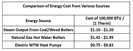
Given that fuel costs will likely only continue to rise, but that, while a new boiler was needed, there was no obvious source of funds to pay for it, a number of options were considered. It is interesting to note, in the following table, the costs of the current coal:wood system. (60% coal), relative to those of the proposed water to water (WTW) heat pumps that are being proposed.
Figure 1. Comparison of the useful energy (upper circled numbers) to the input energy at the MST Power Plant. (MST)
Given that fuel costs will likely only continue to rise, but that, while a new boiler was needed, there was no obvious source of funds to pay for it, a number of options were considered. It is interesting to note, in the following table, the costs of the current coal:wood system. (60% coal), relative to those of the proposed water to water (WTW) heat pumps that are being proposed.
 Figure 2. Comparative Energy costs relative to the current system. (MST)
To digress a little, for their part in addressing a similar problem, the University of Missouri at the Columbia campus is installing a bubbling fluidized bed boiler. The boiler will use biomass to be to displace about 25% of the coal use on campus. The $75 million project has just been completed. However, as I noted in an earlier post, there may be unrecognized processing costs for the biomass which may eat into the campus savings. And while MS&T are looking for ways of handling the now unnecessary smoke stacks, the biomass facility in Columbia has just added three 110-ft tall silos to handle the feed.
Figure 2. Comparative Energy costs relative to the current system. (MST)
To digress a little, for their part in addressing a similar problem, the University of Missouri at the Columbia campus is installing a bubbling fluidized bed boiler. The boiler will use biomass to be to displace about 25% of the coal use on campus. The $75 million project has just been completed. However, as I noted in an earlier post, there may be unrecognized processing costs for the biomass which may eat into the campus savings. And while MS&T are looking for ways of handling the now unnecessary smoke stacks, the biomass facility in Columbia has just added three 110-ft tall silos to handle the feed.
 Figure 3. The polyethylene tubing and the metal end fixtures for insertion into the MS&T boreholes. (MST)
With this encouragement there was an initial discussion of the system in Mid-September 2010, the scheme was approved by the Board of Curators in November 2010, and 2011 was spent in bidding and awarding the contracts and pre-ordering materials. The first day of drilling was on June 4, 2012, just after the Spring Semester. In order to complete the parking lots – to the degree possible – several drill rigs were used at once:
Figure 3. The polyethylene tubing and the metal end fixtures for insertion into the MS&T boreholes. (MST)
With this encouragement there was an initial discussion of the system in Mid-September 2010, the scheme was approved by the Board of Curators in November 2010, and 2011 was spent in bidding and awarding the contracts and pre-ordering materials. The first day of drilling was on June 4, 2012, just after the Spring Semester. In order to complete the parking lots – to the degree possible – several drill rigs were used at once:
 Figure 4. The use of multiple rigs to speed operations (how many?) (MST)
Once a well had been drilled, and the pipes installed, the holes were backfilled with a grout that included significant quantities of sand, to improve the heat transfer. And the two pipes were all that were left protruding.
Figure 4. The use of multiple rigs to speed operations (how many?) (MST)
Once a well had been drilled, and the pipes installed, the holes were backfilled with a grout that included significant quantities of sand, to improve the heat transfer. And the two pipes were all that were left protruding.
 Figure 5. After pipe installation (MST)
Trenches were then cut across the lot to allow the distribution and collection network of pipes to be installed. Once the field connections were fused together, the lines were connected to larger transport pipes at the end of the field, and set into a deeper trench.
Figure 5. After pipe installation (MST)
Trenches were then cut across the lot to allow the distribution and collection network of pipes to be installed. Once the field connections were fused together, the lines were connected to larger transport pipes at the end of the field, and set into a deeper trench.
 Figure 6. The connections between the wells and the distribution network. (MST)
The larger pipes were used to carry the water from each field to the heat exchanger/chiller plant, with three plants being located around the campus. All that then remained was to backfill the trenches, tarmac the lots again, and the campus began to return to normal. The last well did not get drilled until half-way through this semester, but the lots are now coming back into use.
Figure 6. The connections between the wells and the distribution network. (MST)
The larger pipes were used to carry the water from each field to the heat exchanger/chiller plant, with three plants being located around the campus. All that then remained was to backfill the trenches, tarmac the lots again, and the campus began to return to normal. The last well did not get drilled until half-way through this semester, but the lots are now coming back into use.
 Figure 7. Overall layout of the three circuits being used on campus (MST)
With most of the work done on the fields, the remaining work involves the integration of the system into the existing infrastructure, and the necessary changes to the hardware in the various buildings to handle the different ways in which energy is used within them. Much of this change is required since the heating has been, in the past, using steam lines, and these have now to be replaced with the hot water circuit.
Figure 7. Overall layout of the three circuits being used on campus (MST)
With most of the work done on the fields, the remaining work involves the integration of the system into the existing infrastructure, and the necessary changes to the hardware in the various buildings to handle the different ways in which energy is used within them. Much of this change is required since the heating has been, in the past, using steam lines, and these have now to be replaced with the hot water circuit.

The new boiler, which was retrofitted to the university’s existing heating duct system, is expected to produce 150,000 pounds of steam per hour, increasing the 67-year-old power plant’s steam output by 30,000 pounds per hour, and use an estimated 100,000 tons of in-state renewable energy sources such as chipped hardwoods and wood waste.Back at MS&T the number for the heat pump came in part from a WTW heat recovery chiller that the campus had installed in October 2007, and which was saving the campus some $1,500 a day by allowing some of the recovered heat to be produced in useful form. When the campus first looked at the potential they were also able to look at the experience of places such as the Richard Stockton College of New Jersey, which installed a system in 1996. Their installation pioneered many of the decisions made in subsequent operations.
The wells are located on a grid and spaced roughly 15 feet apart. Within each four inch borehole, the installers placed two 1.25 inch diameter high density polyethylene pipes with a U-shaped coupling at the bottom. After the pipes were installed, the boreholes were backfilled with clay slurry to seal them and to enhance heat exchange. In total, the loop system includes 64 miles of heat exchange pipe. In addition, 18 observation wells were located in and around the well field for long-term observation of ground water conditions. The individual wells are connected to 20 four inch diameter lateral supply and return pipes. The laterals, in turn, run to a building at the edge of the field where they are combined into 16 inch primary supply and return lines. These lines are connected to the heat pumps which serve Stockton’s buildings. In the heating mode, the loop serves as a heat source and, in the cooling mode, as a heat sink. The heat pumps range in size from 10 to 35 tons. All are equipped for with air economizers. The equipment is controlled by a building management system using 3,500 data points. This allows the College to take advantage of energy saving options such as duty cycling, night setback and time of day scheduling. The building management system also identifies maintenance needs in the system. . . . . . The system immediately demonstrated that it could carry the entire planned heating load. In the first few years of operation, the average temperature of the well field has drifted upward by several degrees. This occurred because the buildings use more air conditioning than heating. . . . . . Because of the constant changes to the system, and other energy conservation steps, it was difficult to verify energy savings exactly. Based on extensive monitoring, the predictions turned out to be quite accurate.


Read more!
Tuesday, November 6, 2012
The Red Paint People, Doggerland and my DNA.
Over the last couple of months I have been putting up the occasional post on my own family tree, as it is becoming defined by DNA analysis, and at the same time have been looking at some of the early arrivals of Indians in Maine and the North East American continent. (My interest in the latter was initiated by the question of when Europeans first arrived on the continent in enough numbers to influence facial features of the locals).
Two weeks ago I was fortunate to be able to attend a lecture by Bruce Bourque, the Curator of Archaeology at Maine State Museum, and the authority on the Red Paint People, of whom I have written earlier with a follow-up post on their travels. His talk, and the book he just recently released (The Swordfish Hunters) provides much more detail on a people that have largely been neglected by “the archaeologists of Harvard,” who have tended to disregard significant developments this far north of Boston.
The Red Paint People are also called “the Moorehead Phase”, after Warren Moorehead, who first identified them as the “Red Paint” people, because of their custom of burying red ocher with the bodies in their cemeteries. They flourished in a small part of Maine, and their cemeteries have been found along the banks of local rivers. There is, however considerable evidence that they harvested fish and sea-food (their cemeteries have been found in large shell middens), with a peculiarity that they also hunted, ate and used the bones and rostra (the “sword”) of local swordfish. The latter, in particular, was used to provide a stiffened mount behind the harpoon and spear tips used in hunting. They appear to be the first to hunt swordfish, which would have been a dangerous prey for early Holocene man, since they have a nasty habit of attacking the boats of those who have just stabbed them with a harpoon.
 Figure 1. Red Paint Cemeteries in North-East America (The Swordfish Hunters)
The book is a fascinating story of detective work, and archaeology as it builds a picture of a people that began around 5,000 years ago and suddenly disappeared around 3,800 years ago. Dr. Bourque points to evidence that it does not fit within an overall unified culture which has been described as the Maritime Archaic, but rather stands on its own, and emerges from the “Small Stemmed Point” tradition that preceded it. But is totally separate from the Ceramic period that follows.
One of the intriguing parts of the story lies in the thousand-mile link with the Ramah Peninsula in Labrador, that I discussed in a previous post, and Dr. Bourque also points to close similarities between the findings in Maine, and those at the Port au Choix site. One identifying characteristic lies in the development of stone gouges, for use in hollowing out the inside of dugout canoes.
Figure 1. Red Paint Cemeteries in North-East America (The Swordfish Hunters)
The book is a fascinating story of detective work, and archaeology as it builds a picture of a people that began around 5,000 years ago and suddenly disappeared around 3,800 years ago. Dr. Bourque points to evidence that it does not fit within an overall unified culture which has been described as the Maritime Archaic, but rather stands on its own, and emerges from the “Small Stemmed Point” tradition that preceded it. But is totally separate from the Ceramic period that follows.
One of the intriguing parts of the story lies in the thousand-mile link with the Ramah Peninsula in Labrador, that I discussed in a previous post, and Dr. Bourque also points to close similarities between the findings in Maine, and those at the Port au Choix site. One identifying characteristic lies in the development of stone gouges, for use in hollowing out the inside of dugout canoes.
 Figure 2. A Stone Gouge from Maine, and an artist’s rendition of how it would be hafted. (The Swordfish Hunters).
The gouges, as the book argues, show that the Red Paint Peoples were building substantial canoes and boats around 4,000 years ago, that were substantial enough for voyages of a thousand miles, and that this would also make them viable for use in harpooning swordfish (an art in itself as the book illustrates).
The climate change around the time that this culture was flourishing in Maine is not seriously discussed in the book, but I think that it is worth looking at, in context, because it ties in a little with what was happening across the Atlantic, where the culture that built Stonehenge had moved into Britain.
Figure 2. A Stone Gouge from Maine, and an artist’s rendition of how it would be hafted. (The Swordfish Hunters).
The gouges, as the book argues, show that the Red Paint Peoples were building substantial canoes and boats around 4,000 years ago, that were substantial enough for voyages of a thousand miles, and that this would also make them viable for use in harpooning swordfish (an art in itself as the book illustrates).
The climate change around the time that this culture was flourishing in Maine is not seriously discussed in the book, but I think that it is worth looking at, in context, because it ties in a little with what was happening across the Atlantic, where the culture that built Stonehenge had moved into Britain.
 Figure 3. Climate swings in the Northern Hemisphere over the past 10,000 years (the Holocene) (Consulting Geologist)
The significance of these temperature variations is often significantly discounted as climate scientists today would rather emphasize the point of the effects imposed by man, rather than the natural effects we cannot control. Yet the higher temperatures that did exist, even as recently as the last (Medieval) Warming Period are evidenced, for example, by the recent uncovering of an Eskimo village which has been buried under a glacier for the past 500 years. The inhabiting tribe of Yup’ik Eskimo lived, among other things, on caribou and lived at Quinhagak in Alaska. Without the protective ice cap that has covered the site from the time that the Yup’ik left there at the beginning of the Little Ice Age, the site is now rapidly being eroded into the Bering Sea (a fate that is similarly threatening the sites in Maine, where coastal erosion and sea level changes have covered most of the Red Paint People’s locations). But it indicates that we are only now reaching the temperatures at that site that prevailed in the Medieval Warming Period.
The Red Paint People lived at the beginning of what is now referred to as the Minoan Warming Period. And, from data obtained from the Greenland Ice Cores, it is possible to note a couple of facts about the time that the tribe appears to have vanished. First, if the temperatures, as derived from the Ice cores recovered from Greenland are examined in a little more detail:
Figure 3. Climate swings in the Northern Hemisphere over the past 10,000 years (the Holocene) (Consulting Geologist)
The significance of these temperature variations is often significantly discounted as climate scientists today would rather emphasize the point of the effects imposed by man, rather than the natural effects we cannot control. Yet the higher temperatures that did exist, even as recently as the last (Medieval) Warming Period are evidenced, for example, by the recent uncovering of an Eskimo village which has been buried under a glacier for the past 500 years. The inhabiting tribe of Yup’ik Eskimo lived, among other things, on caribou and lived at Quinhagak in Alaska. Without the protective ice cap that has covered the site from the time that the Yup’ik left there at the beginning of the Little Ice Age, the site is now rapidly being eroded into the Bering Sea (a fate that is similarly threatening the sites in Maine, where coastal erosion and sea level changes have covered most of the Red Paint People’s locations). But it indicates that we are only now reaching the temperatures at that site that prevailed in the Medieval Warming Period.
The Red Paint People lived at the beginning of what is now referred to as the Minoan Warming Period. And, from data obtained from the Greenland Ice Cores, it is possible to note a couple of facts about the time that the tribe appears to have vanished. First, if the temperatures, as derived from the Ice cores recovered from Greenland are examined in a little more detail:
 Figure 4. Temperatures in the region over the last 5,000 years (from the Greenland GISP2 Ice core)
Perhaps more to the point, if the extent of sea ice at the time is considered (from the same source) it fell to an historic low during the Minoan.
Figure 4. Temperatures in the region over the last 5,000 years (from the Greenland GISP2 Ice core)
Perhaps more to the point, if the extent of sea ice at the time is considered (from the same source) it fell to an historic low during the Minoan.
 Figure 5. Sea Ice extent over the Holocene (The Ice Chronicles ) (Note the plot has been flipped, relative to the original, in order to conform to the consistency of showing the older period to the left of the plot in the rest of the post).
With this considerable warming the ice retreated from the shores of Greenland, and it became an even more hospitable place that it was at the time almost 3,000 years later when Erik the Red came calling. This warming had another consequence, because it led to a steady rise in the levels of the sea. This is shown in the book as it affects Maine, important since it shows how the shoreline dwellings from the period have since been inundated.
Figure 5. Sea Ice extent over the Holocene (The Ice Chronicles ) (Note the plot has been flipped, relative to the original, in order to conform to the consistency of showing the older period to the left of the plot in the rest of the post).
With this considerable warming the ice retreated from the shores of Greenland, and it became an even more hospitable place that it was at the time almost 3,000 years later when Erik the Red came calling. This warming had another consequence, because it led to a steady rise in the levels of the sea. This is shown in the book as it affects Maine, important since it shows how the shoreline dwellings from the period have since been inundated.
 Figure 6. Sea levels off the coast of Maine over the Holocene (The Swordfish Hunters)
But in Europe that sea rise from the beginning of the Holocene had another consequence. It flooded the land-bridge (known as Doggerland) between what became the isle of Britain and the continent.
Within the British Isles, by 4,000 BP the country had been colonized for about a thousand years by the arrival of an agricultural movement that displaced the earlier hunter-gatherers and, in turn. rapidly changed from a “slash and burn” land clearance into the development of a “celtic arrangement of fields. Colin Burgess in "The Age of Stonehenge" has noted that the settlements towards the end of that transition were already being constructed defensively.
Figure 6. Sea levels off the coast of Maine over the Holocene (The Swordfish Hunters)
But in Europe that sea rise from the beginning of the Holocene had another consequence. It flooded the land-bridge (known as Doggerland) between what became the isle of Britain and the continent.
Within the British Isles, by 4,000 BP the country had been colonized for about a thousand years by the arrival of an agricultural movement that displaced the earlier hunter-gatherers and, in turn. rapidly changed from a “slash and burn” land clearance into the development of a “celtic arrangement of fields. Colin Burgess in "The Age of Stonehenge" has noted that the settlements towards the end of that transition were already being constructed defensively.
 Figure 7. The location of Doggerland about 7000 BP (Bryony Coles via doggerland)
My Y-chromosome has been designated as R1b1b2a1a1d*, which is a variety of Celt, that, as I have mentioned in an earlier post, had come down from Cro-Magnon man. The analysis that has evolved over the past few years (apparently starting at 23andme suggests that this a “Freisian” variety of Celt and there is a body of thought moving to the conclusion that they were the inhabitants of Doggerland that were driven to Britain when the final inundation occurred around 5500 years ago, just before the first circles at Stonehenge were constructed. (And here I now discover that maybe I wasn’t the first of my lineage to work on a Stonehenge).
The first circles at Stonehenge were developed about 5,000 years ago (at the left side of Figure 4). But around 2150 BC or some 4000 BP the Beaker People arrived. In contrast with those, maybe us, who had first developed the site and were moon worshipers, they worshiped the sun. What made the Stonehenge site become what it did was that the simple markers already there to align critical lunar phases could, by moving around the circle ninety degrees, also align to the major solar alignments at mid-winter, mid-summer etc. The ruling elites of the time became more powerful, and with the warmer climes helping sustain agricultural production, society became more static. And the more powerful had enough manpower available to develop, over the next millennium or so, the full glory that became Stonehenge. They also grew into the Wessex Culture with its elaborate and rich graves.
The Beaker People were Celts and still, at the beginning of this time, used stone axes and flint-shaped arrowheads. But copper daggers are found even in the earliest graves and this was the time where the culture was moving into the Bronze Age in Britain, some time after it had developed elsewhere in Europe.
Given that the Red Paint People were aware of native copper deposits, (and were starting to make small ornaments with them) had they known of the metal forming traditions developing in Europe then metal objects would have shown up in the graves. They did not, and even to the time of Champlain stone tools were in use.
So it is logical to conclude that seafaring though the cultures were on both sides of the Atlantic they did not communicate at this time, at least not well enough to teach metal craft, at a time when it might have been easier to travel, from one side of the Atlantic to the other. On the other hand, it might be possible to conjecture an explanation for the long and narrow bayonet points which Dr. Bourque points out as a significant feature of Red Paint burials. He notes that these are too weak to have any great utilitarian value in society, because they were made of stone. He therefore suggests that they had only a ceremonial aspect that has been lost. But it could be that they were an attempt to copy the spear heads that were beginning to be developed in Britain at the time, but which were made utilitarian only by being made of metal. And that would suggest some form of communication between the two societies.
There remain a couple of additional thoughts, both about the ability of early societies such as these to travel long distances, and the mysterious disappearance of whole societal segments. But they arise in events in Greenland that happened during the Medieval Warming Period; the migration of the Thule from Alaska to Northern Greenland in 1000 AD, and the abandonment of the Western Settlement of the Viking in Greenland. Since this is a different time period I will therefore leave those topics to a subsequent post.
Figure 7. The location of Doggerland about 7000 BP (Bryony Coles via doggerland)
My Y-chromosome has been designated as R1b1b2a1a1d*, which is a variety of Celt, that, as I have mentioned in an earlier post, had come down from Cro-Magnon man. The analysis that has evolved over the past few years (apparently starting at 23andme suggests that this a “Freisian” variety of Celt and there is a body of thought moving to the conclusion that they were the inhabitants of Doggerland that were driven to Britain when the final inundation occurred around 5500 years ago, just before the first circles at Stonehenge were constructed. (And here I now discover that maybe I wasn’t the first of my lineage to work on a Stonehenge).
The first circles at Stonehenge were developed about 5,000 years ago (at the left side of Figure 4). But around 2150 BC or some 4000 BP the Beaker People arrived. In contrast with those, maybe us, who had first developed the site and were moon worshipers, they worshiped the sun. What made the Stonehenge site become what it did was that the simple markers already there to align critical lunar phases could, by moving around the circle ninety degrees, also align to the major solar alignments at mid-winter, mid-summer etc. The ruling elites of the time became more powerful, and with the warmer climes helping sustain agricultural production, society became more static. And the more powerful had enough manpower available to develop, over the next millennium or so, the full glory that became Stonehenge. They also grew into the Wessex Culture with its elaborate and rich graves.
The Beaker People were Celts and still, at the beginning of this time, used stone axes and flint-shaped arrowheads. But copper daggers are found even in the earliest graves and this was the time where the culture was moving into the Bronze Age in Britain, some time after it had developed elsewhere in Europe.
Given that the Red Paint People were aware of native copper deposits, (and were starting to make small ornaments with them) had they known of the metal forming traditions developing in Europe then metal objects would have shown up in the graves. They did not, and even to the time of Champlain stone tools were in use.
So it is logical to conclude that seafaring though the cultures were on both sides of the Atlantic they did not communicate at this time, at least not well enough to teach metal craft, at a time when it might have been easier to travel, from one side of the Atlantic to the other. On the other hand, it might be possible to conjecture an explanation for the long and narrow bayonet points which Dr. Bourque points out as a significant feature of Red Paint burials. He notes that these are too weak to have any great utilitarian value in society, because they were made of stone. He therefore suggests that they had only a ceremonial aspect that has been lost. But it could be that they were an attempt to copy the spear heads that were beginning to be developed in Britain at the time, but which were made utilitarian only by being made of metal. And that would suggest some form of communication between the two societies.
There remain a couple of additional thoughts, both about the ability of early societies such as these to travel long distances, and the mysterious disappearance of whole societal segments. But they arise in events in Greenland that happened during the Medieval Warming Period; the migration of the Thule from Alaska to Northern Greenland in 1000 AD, and the abandonment of the Western Settlement of the Viking in Greenland. Since this is a different time period I will therefore leave those topics to a subsequent post.


A more recent unmarked burial pit at Fengate contained three disarticulated burials and one, crouched, the latter with a leaf-shaped arrowhead still sticking between the eighth and ninth ribs.The warmer clime was conducive to the spread of agriculture and an increasing density of population. The cutting of the land bridge, and the slow flooding of what later became the Dogger Bank, in the North Sea, had a personal consequence.

Read more!
Friday, November 2, 2012
Waterjetting 3a - Pump pressure is not cutting pressure
When I began this series I pointed out that whenever a waterjet is going to be used both the target material and the waterjet delivery system have to be considered, if the work is to be done well.
In the last four posts (set 2 in the series) I have tried to emphasize the role of cracks and flaws in the way in which water penetrates into and removes material. It is easier to see this with large-scale operations, such as in the removal of large volumes of soil, but it equally holds true in the abrasive cutting of glass. Now in set 3 the focus is going to swing back to the ways in which high-pressure waterjets are developed, particularly in the different choices of equipment that can be used.
Because this series is meant to help folk understand how systems work, and through that, how to improve production and quality it will tend to shy away from putting a lot of formulae into the presentations. There is a reason that I, an academic, don’t like having students learn equations by rote. It is that it becomes, quite possible, to misremember them. If you are used to looking them up (particularly true in today’s computer world where formulae can easily be used to generate tables) then you are less likely to mis-remember the exact relationships, and to make a possible critical mistake.
But, as I showed in the third post, when the tables of jet flow, horsepower and thrust were generated, there are a few, critical equations that need to be born in mind. And the one that underlies the economics of many operations is tied up in the size of the power that is available to do the work. The basic power equation itself is relatively straightforward:
 Equation 1. Relationship between hydraulic horsepower, pressure and flow.
But the calculation gives different values, depending on where the calculation is made in a circuit. To demonstrate this, let us use a very simple drawing of a flow circuit.
Equation 1. Relationship between hydraulic horsepower, pressure and flow.
But the calculation gives different values, depending on where the calculation is made in a circuit. To demonstrate this, let us use a very simple drawing of a flow circuit.
 Figure 2. The components of a simple flow circuit. Water is drawn from the water tank, through the pump and delivered down a hose to a high-pressure lance, where the water is fed, through a nozzle and aimed at the target, where it does the work.
In the course of this small set of posts the different components that make up this circuit are going to be discussed in turn. But at the end of the first set I mentioned that in an early comparison of the relative cleaning performance of 10,000 psi waterjets of nominally equal power, and flow (10 gpm IIRC) there was a dramatic difference in the cleaning efficiency, as the Navy reported at the time.
Figure 2. The components of a simple flow circuit. Water is drawn from the water tank, through the pump and delivered down a hose to a high-pressure lance, where the water is fed, through a nozzle and aimed at the target, where it does the work.
In the course of this small set of posts the different components that make up this circuit are going to be discussed in turn. But at the end of the first set I mentioned that in an early comparison of the relative cleaning performance of 10,000 psi waterjets of nominally equal power, and flow (10 gpm IIRC) there was a dramatic difference in the cleaning efficiency, as the Navy reported at the time.

Figure 3. Relative cleaning efficiency in areal percentage cleaned, of five competing systems in cleaning heat exchanger tubes in Navy boilers. (Tursi, T.P. Jr., & Deleece, R.J. Jr, (1975) Development of Very High Pressure Waterjet for Cleaning Naval Boiler Tubes, Naval Ship Engineering Center, Philadelphia Division, Philadelphia, PA., 1975, pp. 18.)
Why such a difference? Consider how the power changes from the time that it first enters the pump motor, and then is converted into power along the line to the target. The numbers that I am going to use may seem extreme, but they actually mirror an early experimental set-up in our laboratory, before we learned better. A water flow of 10 gallons a minute (gpm) at a pressure of 10,000 pounds per square inch (psi) pressure will contain – using the above equation; 10,000 x 10/1714 = 58.34 horsepower (hp) But that is the power in the water. Pumps are not 100% efficient, and so there has to be some additional power put into the pump to allow for the relative efficiency of the pump itself. For the sake of illustration let us say that the pump converts the energy at 90% efficiency. Thus the power that is supplied to the drive shaft of the pump will need to be: 58.34/0.9 = 64.8 hp But that is still not the power that we have to supply, since that power – usually – comes from an electric power cord that feeds into a motor, which then, in turn, drives the pump shaft. That motor itself is also not 100% efficient. Let us, for the sake of discussion, say that it is 92.6% efficient. Then the electrical power supplied will be: 64.8/0.926 = 70 hp Now, as the calculation progresses, remember that this is the power that is being paid for. And so, in the first part of the flow, the power is transformed, from electric power to water power, but at the pump.
 Figure 4. The change in power from that input to the motor, to that coming out of the pump.
The water coming out of the pump then flows through either a length of pipe, or high-pressure tubing until it comes to the tool that holds the nozzle. There are a number of different factors that change the flow conditions to the point that it leaves the nozzle. The most critical, and often overlooked, is the size of the hose/tubing that carries the water. Particularly as pumps get larger and more powerful, and the flow rates increase, it is important to ensure that the passage for the water is large enough so that it does not require too much pressure to overcome the friction acting against that flow. I have, myself, put an additional 10-ft length of tubing on a drilling lance, and seen the cutting pressure coming out the end fall from that which drilled a rock at 12 ft/minute to where it could not drill at all. (The pressure drop was around 200 psi per foot). I mentioned in that earlier post that a competitor, running at a pump pressure of 45,000 psi was losing 35,000 psi of that pressure, just to overcome friction in pushing the water down through a tube that was too narrow. As a result the water coming out of the nozzle had barely enough pressure (10,000 psi) to cut into the rock.
At the same time very few people pay a lot of attention to how their nozzle fits on the end of the feed line, or how well it is made. Think of this – you have just spent $200,000 on a system, and yet, because the nozzle is a disposable part, you look around for the cheapest source you can get. You don’t size it for a good fluid fit, nor do you check how well it is machined. And yet the entire performance of your system is controlled by that small item. The difference between a very good nozzle and a standard nozzle can give as much as a factor of 10 improvement on performance – but who checks. The one you use saved you $15 relative to what you would have paid if you had bought the competing product, what a bargain – right?
There are different ways in which pumps operate and produce the high-pressure flow. With a fixed size of orifice in the nozzle and with a given pressure drop along the feed line the pressure at the nozzle will be correspondingly reduced. So that if, for example, we use a 0.063 inch diameter nozzle then the chart you developed after generating the table will show that this will carry a flow of 9.84 gpm at 10,000 psi. But let us suppose that the hose looses 20 psi per foot of length, and that the hose is 200 ft long, then the pressure drop along the hose will be 20 x 200 = 4,000 psi.
Thus the pressure of the water coming out of the hose will be only 6,000 psi. And at an orifice of 0.063 inches, the flow through the orifice will now only be 7.62 gpm. (The way in which the pressure is controlled is assumed to be through bypassing extra flow back to the reservoir through a bleed-off circuit).
Now the pump is still putting out 10 gpm at 10,000 psi, but now the flow out of the nozzle is only 7.62 gpm at 6,000 psi. The power in this jet is (7.62 x 6,000/1714) only 26.7 hp. This is only 38% of the energy going into the pump.
Figure 4. The change in power from that input to the motor, to that coming out of the pump.
The water coming out of the pump then flows through either a length of pipe, or high-pressure tubing until it comes to the tool that holds the nozzle. There are a number of different factors that change the flow conditions to the point that it leaves the nozzle. The most critical, and often overlooked, is the size of the hose/tubing that carries the water. Particularly as pumps get larger and more powerful, and the flow rates increase, it is important to ensure that the passage for the water is large enough so that it does not require too much pressure to overcome the friction acting against that flow. I have, myself, put an additional 10-ft length of tubing on a drilling lance, and seen the cutting pressure coming out the end fall from that which drilled a rock at 12 ft/minute to where it could not drill at all. (The pressure drop was around 200 psi per foot). I mentioned in that earlier post that a competitor, running at a pump pressure of 45,000 psi was losing 35,000 psi of that pressure, just to overcome friction in pushing the water down through a tube that was too narrow. As a result the water coming out of the nozzle had barely enough pressure (10,000 psi) to cut into the rock.
At the same time very few people pay a lot of attention to how their nozzle fits on the end of the feed line, or how well it is made. Think of this – you have just spent $200,000 on a system, and yet, because the nozzle is a disposable part, you look around for the cheapest source you can get. You don’t size it for a good fluid fit, nor do you check how well it is machined. And yet the entire performance of your system is controlled by that small item. The difference between a very good nozzle and a standard nozzle can give as much as a factor of 10 improvement on performance – but who checks. The one you use saved you $15 relative to what you would have paid if you had bought the competing product, what a bargain – right?
There are different ways in which pumps operate and produce the high-pressure flow. With a fixed size of orifice in the nozzle and with a given pressure drop along the feed line the pressure at the nozzle will be correspondingly reduced. So that if, for example, we use a 0.063 inch diameter nozzle then the chart you developed after generating the table will show that this will carry a flow of 9.84 gpm at 10,000 psi. But let us suppose that the hose looses 20 psi per foot of length, and that the hose is 200 ft long, then the pressure drop along the hose will be 20 x 200 = 4,000 psi.
Thus the pressure of the water coming out of the hose will be only 6,000 psi. And at an orifice of 0.063 inches, the flow through the orifice will now only be 7.62 gpm. (The way in which the pressure is controlled is assumed to be through bypassing extra flow back to the reservoir through a bleed-off circuit).
Now the pump is still putting out 10 gpm at 10,000 psi, but now the flow out of the nozzle is only 7.62 gpm at 6,000 psi. The power in this jet is (7.62 x 6,000/1714) only 26.7 hp. This is only 38% of the energy going into the pump.
 Figure 5. The power losses to the nozzle.
Unfortunately this is not the end of the losses. Particularly in cleaning operations ther is a tendency for the operator to hold the nozzle at a comfortable distance from the target, so that the effect can be seen. But, as I will show in later posts, the jet pressure can fall rapidly as stand-off distance increases, particularly with a poor nozzle. A good range for a normal nozzle in a cleaning operation is about 125 nozzle diameters. So that at a diameter of 0.063 inches this range is less than 8 inches. Many people hold the nozzle at least a foot from the target.
If the nozzle is held about that far from the target the pressure will have fallen by perhaps 65%. The water thus reaches the target at around 2,000 psi. The flow rate is 7.62 gpm, and the actual horsepower of the water doing the work is 8.89 hp. This is 12.7% of the power that is being paid for through the meter. And the unfortunate problem is that no-one can tell, just by looking at the jet, what the pressure and flow rates are. So that often these losses go undetected, and folk merely complain about how the target material is more resistant today, not recognizing that they are throwing away 87% of the power that they are paying for.
Figure 5. The power losses to the nozzle.
Unfortunately this is not the end of the losses. Particularly in cleaning operations ther is a tendency for the operator to hold the nozzle at a comfortable distance from the target, so that the effect can be seen. But, as I will show in later posts, the jet pressure can fall rapidly as stand-off distance increases, particularly with a poor nozzle. A good range for a normal nozzle in a cleaning operation is about 125 nozzle diameters. So that at a diameter of 0.063 inches this range is less than 8 inches. Many people hold the nozzle at least a foot from the target.
If the nozzle is held about that far from the target the pressure will have fallen by perhaps 65%. The water thus reaches the target at around 2,000 psi. The flow rate is 7.62 gpm, and the actual horsepower of the water doing the work is 8.89 hp. This is 12.7% of the power that is being paid for through the meter. And the unfortunate problem is that no-one can tell, just by looking at the jet, what the pressure and flow rates are. So that often these losses go undetected, and folk merely complain about how the target material is more resistant today, not recognizing that they are throwing away 87% of the power that they are paying for.
 Figure 6. Power losses from the power cord to the target.
One of the objects of this series is to help reduce these losses, by avoiding those mistakes that those of us who started in the industry some 40-odd years ago made all the time.
Figure 6. Power losses from the power cord to the target.
One of the objects of this series is to help reduce these losses, by avoiding those mistakes that those of us who started in the industry some 40-odd years ago made all the time.


Figure 3. Relative cleaning efficiency in areal percentage cleaned, of five competing systems in cleaning heat exchanger tubes in Navy boilers. (Tursi, T.P. Jr., & Deleece, R.J. Jr, (1975) Development of Very High Pressure Waterjet for Cleaning Naval Boiler Tubes, Naval Ship Engineering Center, Philadelphia Division, Philadelphia, PA., 1975, pp. 18.)
Why such a difference? Consider how the power changes from the time that it first enters the pump motor, and then is converted into power along the line to the target. The numbers that I am going to use may seem extreme, but they actually mirror an early experimental set-up in our laboratory, before we learned better. A water flow of 10 gallons a minute (gpm) at a pressure of 10,000 pounds per square inch (psi) pressure will contain – using the above equation; 10,000 x 10/1714 = 58.34 horsepower (hp) But that is the power in the water. Pumps are not 100% efficient, and so there has to be some additional power put into the pump to allow for the relative efficiency of the pump itself. For the sake of illustration let us say that the pump converts the energy at 90% efficiency. Thus the power that is supplied to the drive shaft of the pump will need to be: 58.34/0.9 = 64.8 hp But that is still not the power that we have to supply, since that power – usually – comes from an electric power cord that feeds into a motor, which then, in turn, drives the pump shaft. That motor itself is also not 100% efficient. Let us, for the sake of discussion, say that it is 92.6% efficient. Then the electrical power supplied will be: 64.8/0.926 = 70 hp Now, as the calculation progresses, remember that this is the power that is being paid for. And so, in the first part of the flow, the power is transformed, from electric power to water power, but at the pump.


Read more!
OGPSS - The quiet steps of a Geothermal movement
The election is now less than a week away, with two entirely different paths possible for our future as we move past the election into next year. The two approaches to energy are particularly different, but it is pointless to do any further comparison, since the airwaves have (on the rare occasion that these differences are explored) discussed these from all points on the spectrum. But nevertheless it gives an occasion to step aside from Iran, for a week, and to draw your attention to something you may have missed in all this debate, and yet is starting to happen on University campuses that are scrambling to meet that ever rising fuel bill.
In the current debate both sides seem to anticipate that the energy future is rosy. As an illustration, I was struck by a comment just this last week:
 Figure 1. Production from the Haynesville Shale in Louisiana (Go Haynesville Shale )
Now there are a variety of reasons for the decline, a significant one being that the number of wells being drilled has fallen dramatically, as the article recognizes. But that is itself, in part, a recognition of the current economics of the business. I had a discussion, just this past week, with the daughter of an investor who had “lost his shirt” over a natural gas well investment. The difference between the hype and the reality is disturbing, and does not bode well for a stable future. Which poses the question as to what the reality of that future might be?
I live in Missouri, and a number of years ago colleagues of mine evaluated the potential benefits of renewable energy and were left severely unimpressed with the potential for wind and solar in this state. At the time I was not sure what the answer for our state was.
The campus where I worked until I retired, (Missouri University of Science and Technology – the new UMR) had been quite revolutionary some decades ago in starting to burn wood with coal, both as a way of controlling emissions and costs. Now those benefits were disappearing and the campus faced the prospect of finding about $25 million for a new boiler, at a time when state funds are not likely to be available, and which philanthropist wants to fund a boiler? So the campus had to be creative. And it was!
Figure 1. Production from the Haynesville Shale in Louisiana (Go Haynesville Shale )
Now there are a variety of reasons for the decline, a significant one being that the number of wells being drilled has fallen dramatically, as the article recognizes. But that is itself, in part, a recognition of the current economics of the business. I had a discussion, just this past week, with the daughter of an investor who had “lost his shirt” over a natural gas well investment. The difference between the hype and the reality is disturbing, and does not bode well for a stable future. Which poses the question as to what the reality of that future might be?
I live in Missouri, and a number of years ago colleagues of mine evaluated the potential benefits of renewable energy and were left severely unimpressed with the potential for wind and solar in this state. At the time I was not sure what the answer for our state was.
The campus where I worked until I retired, (Missouri University of Science and Technology – the new UMR) had been quite revolutionary some decades ago in starting to burn wood with coal, both as a way of controlling emissions and costs. Now those benefits were disappearing and the campus faced the prospect of finding about $25 million for a new boiler, at a time when state funds are not likely to be available, and which philanthropist wants to fund a boiler? So the campus had to be creative. And it was!
 Figure 2. Old Campus Power Plant - the question of what to do with the stacks is unresolved.
Starting in the summer of 2010 the campus proposed the use of a ground-source heat pump system as a method of using the Geothermal potential under the campus to lower the overall operating costs of generating power, while at the same time addressing issues regarding the generation of carbon dioxide, and the use of large volumes of water that are one of the costs of conventional coal-fired boiler use.
The initial proposal was approved in remarkable time and over the past summer drilling crews moved in for the initial drilling of the wells. Unfortunately (but realistically) the greatest amount of open space around campus that can be used are the parking lots. And so s number of drilling rigs appeared as the students left for the summer, and proceeded to drill a series of roughly 600 wells, each around 400 ft deep. The last was completed last month, and the wells were then lined with piping and are currently being connected into a triad of networks.
Figure 2. Old Campus Power Plant - the question of what to do with the stacks is unresolved.
Starting in the summer of 2010 the campus proposed the use of a ground-source heat pump system as a method of using the Geothermal potential under the campus to lower the overall operating costs of generating power, while at the same time addressing issues regarding the generation of carbon dioxide, and the use of large volumes of water that are one of the costs of conventional coal-fired boiler use.
The initial proposal was approved in remarkable time and over the past summer drilling crews moved in for the initial drilling of the wells. Unfortunately (but realistically) the greatest amount of open space around campus that can be used are the parking lots. And so s number of drilling rigs appeared as the students left for the summer, and proceeded to drill a series of roughly 600 wells, each around 400 ft deep. The last was completed last month, and the wells were then lined with piping and are currently being connected into a triad of networks.
 Figure 3. Simplified illustration of the geothermal circuit.
Basically the system works on the idea that the ground, in depth, is at a relatively constant temperature. (For those of us who have mined in depth the old rule of thumb in the Northern UK was 60 deg at 60 ft and 1 degree rise per 60 ft thereafter – but the geothermal gradient varies around the world). Given this relatively consistent temperature, in winter the cool water (the blue line) can be pumped underground, heated and returned through the red line, from which it passes through a heat exchanger system that provides heat to the campus, while then being returned via the blue line to repeat the process.
In the summer the flow is reversed. The hot water from the heat exchanger/chiller is returned to the wells through the red lines, releasing the heat into the ground and cooling before it returns back to the surface through the blue line, and into the chiller/heat exchanger to provide a cooling source for the campus.
Current estimates are that the initial costs (paid for with a bond issue) will be no more than the cost of that boiler (which wasn’t going to be funded, yet was needed), but that the campus will save, in the beginning, some $1 million in energy costs (the remaining energy will be supplied with natural gas and the boilers will be retired in 2014) and this will service the bond. The funds only allow some 60% of the campus to be initially served, through three separate plants that are set around the campus. In time, as savings mount, it is likely that other buildings will be brought into the loop (though some have sufficiently antiquated heating and cooling systems that the entire building will need renovation first.
Over the lifetime of the system (and there is not a lot of fragile equipment in the loop, so this may be more than 50-years) energy savings are likely to rise to more than $3 million a year, as the energy crisis that we are currently pretending isn’t coming finally comes to pass.
Given the benefits that the system will develop it is not surprising that MS&T are not alone in this approach. In fact they learned of the concept at the time that Ball State was beginning their project. That project has just been dedicated and anticipates, being larger than ours, that it will save that campus around $2 million a year. It also includes some 3,600 wells by the time that the second phase of the program is completed.
The idea is beginning to catch on, and there are a small but growing number of campuses now that are in the throes of the same type of effort, though in each case tailored to the individual needs of the different campuses. Hampton University in Virginia is heating their Multi-Purpose Building, Indiana Tech has restored and powered a Civil War era building, Montana Tech will use the heat from mine waters underneath the campus. In Boise, ID the ground water temperature is a little higher (around 170 degrees) and the city has used geothermal energy since 1983, and now Boise State is joining in with its own plant. As with the Montana project, so the program at New Mexico Tech has also been funded as part of the Recovery Act. Some of the potential benefits of that program have been described by the Department of Energy. However that presentation also illustrates the transience of the funding opportunity.
Figure 3. Simplified illustration of the geothermal circuit.
Basically the system works on the idea that the ground, in depth, is at a relatively constant temperature. (For those of us who have mined in depth the old rule of thumb in the Northern UK was 60 deg at 60 ft and 1 degree rise per 60 ft thereafter – but the geothermal gradient varies around the world). Given this relatively consistent temperature, in winter the cool water (the blue line) can be pumped underground, heated and returned through the red line, from which it passes through a heat exchanger system that provides heat to the campus, while then being returned via the blue line to repeat the process.
In the summer the flow is reversed. The hot water from the heat exchanger/chiller is returned to the wells through the red lines, releasing the heat into the ground and cooling before it returns back to the surface through the blue line, and into the chiller/heat exchanger to provide a cooling source for the campus.
Current estimates are that the initial costs (paid for with a bond issue) will be no more than the cost of that boiler (which wasn’t going to be funded, yet was needed), but that the campus will save, in the beginning, some $1 million in energy costs (the remaining energy will be supplied with natural gas and the boilers will be retired in 2014) and this will service the bond. The funds only allow some 60% of the campus to be initially served, through three separate plants that are set around the campus. In time, as savings mount, it is likely that other buildings will be brought into the loop (though some have sufficiently antiquated heating and cooling systems that the entire building will need renovation first.
Over the lifetime of the system (and there is not a lot of fragile equipment in the loop, so this may be more than 50-years) energy savings are likely to rise to more than $3 million a year, as the energy crisis that we are currently pretending isn’t coming finally comes to pass.
Given the benefits that the system will develop it is not surprising that MS&T are not alone in this approach. In fact they learned of the concept at the time that Ball State was beginning their project. That project has just been dedicated and anticipates, being larger than ours, that it will save that campus around $2 million a year. It also includes some 3,600 wells by the time that the second phase of the program is completed.
The idea is beginning to catch on, and there are a small but growing number of campuses now that are in the throes of the same type of effort, though in each case tailored to the individual needs of the different campuses. Hampton University in Virginia is heating their Multi-Purpose Building, Indiana Tech has restored and powered a Civil War era building, Montana Tech will use the heat from mine waters underneath the campus. In Boise, ID the ground water temperature is a little higher (around 170 degrees) and the city has used geothermal energy since 1983, and now Boise State is joining in with its own plant. As with the Montana project, so the program at New Mexico Tech has also been funded as part of the Recovery Act. Some of the potential benefits of that program have been described by the Department of Energy. However that presentation also illustrates the transience of the funding opportunity.
 Figure 4. The budget for the Geothermal Technologies Program (DOE)
Given that drop in funding, it is yet still possible, given the savings projected not only here but elsewhere, that this technology may still catch on and become more widely adopted. I’ll keep you posted (among other things with more technical details).
Figure 4. The budget for the Geothermal Technologies Program (DOE)
Given that drop in funding, it is yet still possible, given the savings projected not only here but elsewhere, that this technology may still catch on and become more widely adopted. I’ll keep you posted (among other things with more technical details).
"Peak oilers have become almost extinct, destroyed by the arrival of new technologies with the U.S. leading the oil supply change," said David Hufton of oil brokerage PVM.And yet, in the same week I received another newsletter from Go Haynesville Shale predicting (from Seeking Alpha) that 2013 will see the decline in Hanesville production.


Read more!
Subscribe to:
Posts (Atom)

